Sally Kang
why join the navy.
Softmax classifier implementation
Introduction
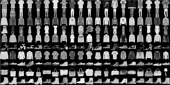
In this post, we are going to build a Softmax classifier to classify fashion MNIST dataset.
Multinomial Logistic Regression
Why
Considering that we are expected to predict a categorical (or discrete) outcome, we have chosen logistic regression as the primary method to perform the tasks.
There are three types of logistic regression:
- Binary Logistic Regression for only two possible outcomes,
- Multinomial Logistic Regression for three or more categories without ordering
- Ordinal Logistic Regression three or more categories with ordering.
In our case, it would be suitable to choose Multinomial Logistic Regression as we are given ten different categories to classify. `0: ‘T - shirt / top’, 1: ‘Trouser’, 2: ‘Pullover’, 3: ‘Dress’, 4: ‘Coat’, 5: ‘Sandal’, 6: ‘Shirt’, 7: ‘Sneaker’, 8: ‘Bag’, 9: ‘Ankleboot’
Mechanism
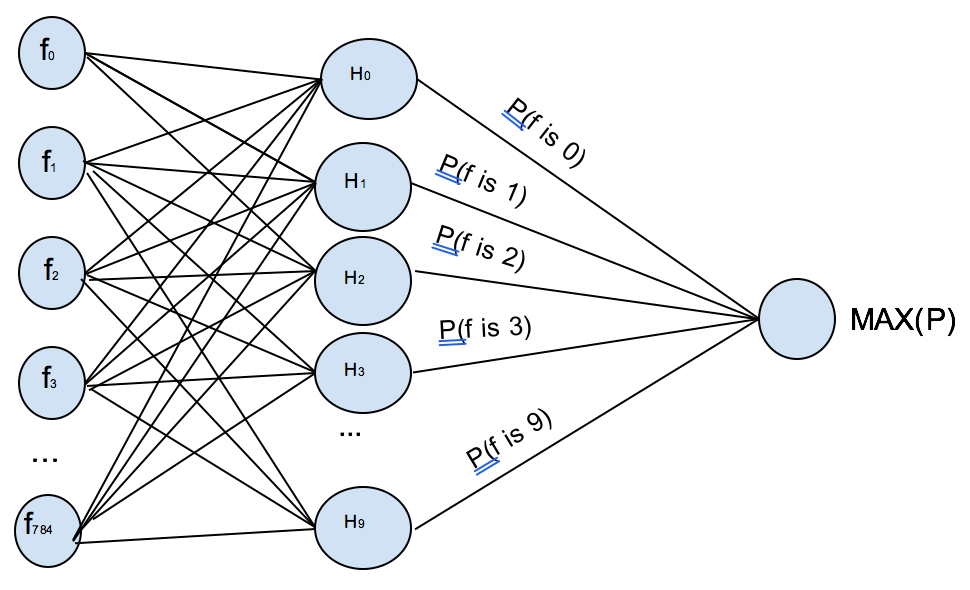
In general, binary logistic regression can be considered as if the logistic function is a single “neuron” that returns the probability that input sample is the target that the neuron was trained to recognize.
To generalize a binary logistic regression to classify ten different categories, we can create a collection of these binary “neurons” with one for each class of the things we want to distinguish. To classify the ten categories 0-9, we would need ten trained models for ten categories to return corresponding probability, and MAX(P) is the result with the highest probability. As shown below:
Softmax Classifier
Loss Function
Softmax classifier is used as the most popular generalization of multiple logistic regression. However, unlike the classifiers like SVM which treats the outputs f(xi,W) of object functions as scores for each class, Softmax classifier would interpret these scores as unnormalized log probabilities for each class label, which means we would use cross-entropy loss function instead of hinge loss function:
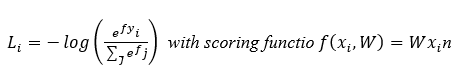
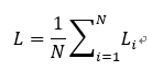
Where the notation f_j is used to mean the j-th element of the vector of class scores f. So, to compute the cross-entropy loss over an entire dataset is done by taking the average:
Here, the function f_j (z)=ⅇ^(z_j )/(Σ_k ⅇ^(z_k ) ) is so called the Softmax function.
Gradient-based Optimization
Hence, now our Softmax classifier aims to minimize the cross-entropy loss as much as possible. In our case, to improve the performance, we evaluate loss function using the gradient descent algorithm instead of the simple grid search.
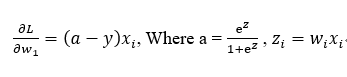
To learn the weight coefficient of Softmax regression model via gradient-based optimization, we compute the partial derivative of the log-likelihood function – w.r.t. the jth weight – as follows:
Regularization
Also, to avoid overfitting, we implement Softmax classifier with L_2 weight decay regularization. That is to define a regularization penalty, a function that operates on our weight matrix W, to help we find better choices of W that will improve our model’s ability to generalize and reduce overfitting. It is common to use “weight decay,” where after each epoch, the weights are multiplied by a factor to prevent from growing too large and can be represented as gradient descent on a quadratic regularization term:
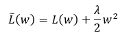
With this regularization parameter, we could trade off the origin loss L with the substantial weights penalization, and ‘w’ is the coefficient of the weight matrix.
Momentum
Considering the model could easily get stuck in, and the algorithm will determine that it has reached the global minima leading to sub-optimal results, we need to implement momentum term in the objective function to get better converge rates. This momentum term is a value between 0 and 1 that increases the size of the steps taken towards the minimum by trying to jump from local minima. Here we can define a momentum, which is a moving average of our gradients. We then use it to update the weight of the network. This could be written as follows:
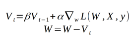 Where L — is loss function, triangular thing — gradient w.r.t weight and alpha — learning rate.
Performance
Here we would take the first 2,000 test examples from given dataset to analyze the performance of our Softmax classifier.
To give an overall performance of each class for further statistics, confusion matrixes generated with our final model are presented below.
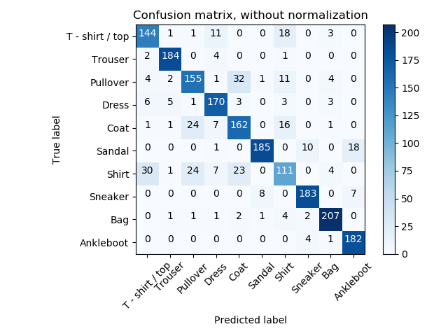
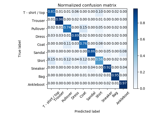
Overall, it shows we have the lowest accuracy of Shirt class, also the second lowest accuracy of Pullover class and the third lowest accuracy of Coat class. With showing these three class in image format, we can find out that they are all upper garment, which means they have more common image features than with other class. This indicates our classifier is not fitted to classify the upper garment type very well. However, the highest accuracies are all come from the shoes and bags types, which means our classifiers are trained to classify objects of accessories shape more efficiently.
Table.1 Accuracies with different number of epochs
| Epochs | Test Accuracy( lr = 0.1) |
|---|---|
| 50 | 79.950 % |
| 150 | 81.700 % |
| 250 | 81.850 % |
| 350 | 82.050 % |
#
Table 2. Accuracies with different learning rates
| Learning Rates | Test Accuracy( lr = 0.1) |
|---|---|
| 0.8 | 83.700 % |
| 0.1 | 82.000 % |
| 0.01 | 75.750 % |
| 0.001 | 66.100 % |
Hope it’s helpful. You can get the source code from my Github repo `